MATLAB练习例子九(微分方程)
返回
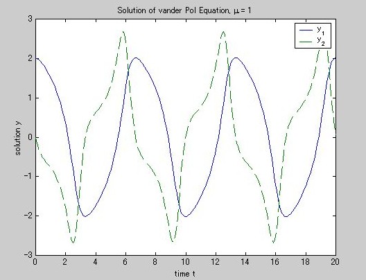
function dydt = vdp1(t,y)
dydt = [y(2); (1-y(1)^2)*y(2)-y(1)];
》 [t,y] = ode45('vdp1',[0 20],[2;0]);
》 plot(t,y(:,1),'-',t,y(:,2),'--')
》 title('Solution of vander Pol Equation, \mu = 1');
》 xlabel('time t');
》 ylabel('solution y');
》 legend('y_1','y_2')
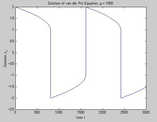
 function dydt = vdp1000(t,y)
dydt = [y(2); 1000*(1-y(1)^2)*y(2)-y(1)];
》 [t,y] = ode15s('vdp1000',[0 3000],[2;0]);
》 plot(t,y(:,1),'-');
》 title('Solution of van der Pol Equation, \mu = 1000');
》 xlabel('time t');
》 ylabel('Solution y_1');
function dydt = vdp1000(t,y)
dydt = [y(2); 1000*(1-y(1)^2)*y(2)-y(1)];
》 [t,y] = ode15s('vdp1000',[0 3000],[2;0]);
》 plot(t,y(:,1),'-');
》 title('Solution of van der Pol Equation, \mu = 1000');
》 xlabel('time t');
》 ylabel('Solution y_1');
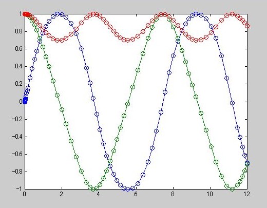
 》 type rigidode.m
function varargout = rigidode(t,y,flag)
%RIGIDODE Euler equations of a rigid body without external forces.
% A standard test problem for non-stiff solvers proposed by Krogh. The
% analytical solutions are Jacobian elliptic functions accessible in
% MATLAB. The interval here is about 1.5 periods; it is that for which
% solutions are plotted on p. 243 of Shampine and Gordon.
%
% RIGIDODE([],[],'init') returns the default TSPAN, Y0, and OPTIONS values
% for this problem. These values are retrieved by an ODE Suite solver if
% the solver is invoked with empty TSPAN or Y0 arguments. This example
% does not set any OPTIONS, so the third output argument is set to empty
% [] instead of an OPTIONS structure created with ODESET.
%
% L. F. Shampine and M. K. Gordon, Computer Solution of Ordinary
% Differential Equations, W.H. Freeman & Co., 1975.
%
% See also ODE45, ODE23, ODE113, ODESET, ODEFILE.
% Mark W. Reichelt and Lawrence F. Shampine, 3-23-94, 4-19-94
% Copyright (c) 1984-98 by The MathWorks, Inc.
% $Revision: 1.8 $ $Date: 1997/11/21 23:27:00 $
switch flag
case '' % Return dy/dt = f(t,y).
varargout{1} = f(t,y);
case 'init' % Return default [tspan,y0,options].
[varargout{1:3}] = init;
otherwise
error(['Unknown flag ''' flag '''.']);
end
% --------------------------------------------------------------------------
function dydt = f(t,y)
dydt = [y(2)*y(3); -y(1)*y(3); -0.51*y(1)*y(2)];
% --------------------------------------------------------------------------
function [tspan,y0,options] = init
tspan = [0; 12];
y0 = [0; 1; 1];
options = [];
》 tspan = [0 12];
》 y0 = [0; 1; 1];
》 ode45('f',tspan,y0);
??? エラー: ==> nargin
正しいM-fileではありません.
エラー: ==> C:\MATLABR11\toolbox\matlab\funfun\ode45.m
行番号: 280 ==>if (exist(odefile) == 3) | (nargin(odefile) == 2) % don't nargin MEX files
》 ode45('rigidode',tspan,y0);
》 type rigidode.m
function varargout = rigidode(t,y,flag)
%RIGIDODE Euler equations of a rigid body without external forces.
% A standard test problem for non-stiff solvers proposed by Krogh. The
% analytical solutions are Jacobian elliptic functions accessible in
% MATLAB. The interval here is about 1.5 periods; it is that for which
% solutions are plotted on p. 243 of Shampine and Gordon.
%
% RIGIDODE([],[],'init') returns the default TSPAN, Y0, and OPTIONS values
% for this problem. These values are retrieved by an ODE Suite solver if
% the solver is invoked with empty TSPAN or Y0 arguments. This example
% does not set any OPTIONS, so the third output argument is set to empty
% [] instead of an OPTIONS structure created with ODESET.
%
% L. F. Shampine and M. K. Gordon, Computer Solution of Ordinary
% Differential Equations, W.H. Freeman & Co., 1975.
%
% See also ODE45, ODE23, ODE113, ODESET, ODEFILE.
% Mark W. Reichelt and Lawrence F. Shampine, 3-23-94, 4-19-94
% Copyright (c) 1984-98 by The MathWorks, Inc.
% $Revision: 1.8 $ $Date: 1997/11/21 23:27:00 $
switch flag
case '' % Return dy/dt = f(t,y).
varargout{1} = f(t,y);
case 'init' % Return default [tspan,y0,options].
[varargout{1:3}] = init;
otherwise
error(['Unknown flag ''' flag '''.']);
end
% --------------------------------------------------------------------------
function dydt = f(t,y)
dydt = [y(2)*y(3); -y(1)*y(3); -0.51*y(1)*y(2)];
% --------------------------------------------------------------------------
function [tspan,y0,options] = init
tspan = [0; 12];
y0 = [0; 1; 1];
options = [];
》 tspan = [0 12];
》 y0 = [0; 1; 1];
》 ode45('f',tspan,y0);
??? エラー: ==> nargin
正しいM-fileではありません.
エラー: ==> C:\MATLABR11\toolbox\matlab\funfun\ode45.m
行番号: 280 ==>if (exist(odefile) == 3) | (nargin(odefile) == 2) % don't nargin MEX files
》 ode45('rigidode',tspan,y0);
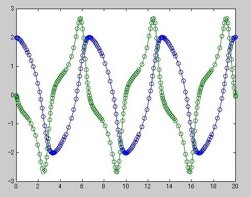
 》 ode15s('vdpode');
》 type vdpode.m
function varargout = vdpode(t,y,flag,mu)
%VDPODE Parameterizable van der Pol equation (stiff for large mu).
% VDPODE(T,Y) or VDPODE(T,Y,[],MU) returns the derivatives vector for the
% van der Pol equation. By default, MU is 1, and the problem is not
% stiff. Optionally, pass in the MU parameter as an additional parameter
% to an ODE Suite solver. The problem becomes more stiff as MU is
% increased.
%
% When MU is 1000 the equation is in relaxation oscillation, and the
% problem becomes very stiff. The limit cycle has portions where the
% solution components change slowly and the problem is quite stiff,
% alternating with regions of very sharp change where it is not stiff
% (quasi-discontinuities). The initial conditions are close to an area of
% slow change so as to test schemes for the selection of the initial step
% size.
%
% VDPODE(T,Y,'jacobian') or VDPODE(T,Y,'jacobian',MU) returns the Jacobian
% matrix dF/dY evaluated analytically at (T,Y). By default, the stiff
% solvers of the ODE Suite approximate Jacobian matrices numerically.
% However, if the ODE Solver property Jacobian is set to 'on' with ODESET,
% a solver calls the ODE file with the flag 'jacobian' to obtain dF/dY.
% Providing the solvers with an analytic Jacobian is not necessary, but it
% can improve the reliability and efficiency of integration.
%
% VDPODE([],[],'init') returns the default TSPAN, Y0, and OPTIONS values
% for this problem (see RIGIDODE). The ODE solver property Vectorized is
% set to 'on' with ODESET because VDPODE is coded so that calling
% VDPODE(T,[Y1 Y2 ...]) returns [VDPODE(T,Y1) VDPODE(T,Y2) ...] for
% scalar time T and vectors Y1,Y2,... The stiff solvers of the ODE Suite
% take advantage of this feature when approximating the columns of the
% Jacobian numerically.
%
% L. F. Shampine, Evaluation of a test set for stiff ODE solvers, ACM
% Trans. Math. Soft., 7 (1981) pp. 409-420.
%
% See also ODE15S, ODE23S, ODESET, ODEFILE.
% Mark W. Reichelt and Lawrence F. Shampine, 3-23-94, 4-19-94
% Copyright (c) 1984-98 by The MathWorks, Inc.
% $Revision: 1.10 $ $Date: 1997/11/21 23:27:28 $
if nargin < 4 | isempty(mu)
mu = 1;
end
switch flag
case '' % Return dy/dt = f(t,y).
varargout{1} = f(t,y,mu);
case 'init' % Return default [tspan,y0,options].
[varargout{1:3}] = init(mu);
case 'jacobian' % Return Jacobian matrix df/dy.
varargout{1} = jacobian(t,y,mu);
otherwise
error(['Unknown flag ''' flag '''.']);
end
% --------------------------------------------------------------------------
function dydt = f(t,y,mu)
dydt = [y(2,:); (mu*(1-y(1,:).^2).*y(2,:) - y(1,:))]; % Vectorized
% --------------------------------------------------------------------------
function [tspan,y0,options] = init(mu)
tspan = [0; max(20,3*mu)]; % several periods
y0 = [2; 0];
options = odeset('Vectorized','on');
% --------------------------------------------------------------------------
function dfdy = jacobian(t,y,mu)
dfdy = [ 0 1
(-2*mu*y(1)*y(2) - 1) (mu*(1-y(1)^2)) ];
》 ode15s('vdpode');
》 type vdpode.m
function varargout = vdpode(t,y,flag,mu)
%VDPODE Parameterizable van der Pol equation (stiff for large mu).
% VDPODE(T,Y) or VDPODE(T,Y,[],MU) returns the derivatives vector for the
% van der Pol equation. By default, MU is 1, and the problem is not
% stiff. Optionally, pass in the MU parameter as an additional parameter
% to an ODE Suite solver. The problem becomes more stiff as MU is
% increased.
%
% When MU is 1000 the equation is in relaxation oscillation, and the
% problem becomes very stiff. The limit cycle has portions where the
% solution components change slowly and the problem is quite stiff,
% alternating with regions of very sharp change where it is not stiff
% (quasi-discontinuities). The initial conditions are close to an area of
% slow change so as to test schemes for the selection of the initial step
% size.
%
% VDPODE(T,Y,'jacobian') or VDPODE(T,Y,'jacobian',MU) returns the Jacobian
% matrix dF/dY evaluated analytically at (T,Y). By default, the stiff
% solvers of the ODE Suite approximate Jacobian matrices numerically.
% However, if the ODE Solver property Jacobian is set to 'on' with ODESET,
% a solver calls the ODE file with the flag 'jacobian' to obtain dF/dY.
% Providing the solvers with an analytic Jacobian is not necessary, but it
% can improve the reliability and efficiency of integration.
%
% VDPODE([],[],'init') returns the default TSPAN, Y0, and OPTIONS values
% for this problem (see RIGIDODE). The ODE solver property Vectorized is
% set to 'on' with ODESET because VDPODE is coded so that calling
% VDPODE(T,[Y1 Y2 ...]) returns [VDPODE(T,Y1) VDPODE(T,Y2) ...] for
% scalar time T and vectors Y1,Y2,... The stiff solvers of the ODE Suite
% take advantage of this feature when approximating the columns of the
% Jacobian numerically.
%
% L. F. Shampine, Evaluation of a test set for stiff ODE solvers, ACM
% Trans. Math. Soft., 7 (1981) pp. 409-420.
%
% See also ODE15S, ODE23S, ODESET, ODEFILE.
% Mark W. Reichelt and Lawrence F. Shampine, 3-23-94, 4-19-94
% Copyright (c) 1984-98 by The MathWorks, Inc.
% $Revision: 1.10 $ $Date: 1997/11/21 23:27:28 $
if nargin < 4 | isempty(mu)
mu = 1;
end
switch flag
case '' % Return dy/dt = f(t,y).
varargout{1} = f(t,y,mu);
case 'init' % Return default [tspan,y0,options].
[varargout{1:3}] = init(mu);
case 'jacobian' % Return Jacobian matrix df/dy.
varargout{1} = jacobian(t,y,mu);
otherwise
error(['Unknown flag ''' flag '''.']);
end
% --------------------------------------------------------------------------
function dydt = f(t,y,mu)
dydt = [y(2,:); (mu*(1-y(1,:).^2).*y(2,:) - y(1,:))]; % Vectorized
% --------------------------------------------------------------------------
function [tspan,y0,options] = init(mu)
tspan = [0; max(20,3*mu)]; % several periods
y0 = [2; 0];
options = odeset('Vectorized','on');
% --------------------------------------------------------------------------
function dfdy = jacobian(t,y,mu)
dfdy = [ 0 1
(-2*mu*y(1)*y(2) - 1) (mu*(1-y(1)^2)) ];
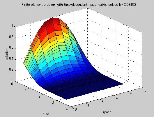
》 type fem1ode
function varargout = fem1ode(t,y,flag,N)
%FEM1ODE Stiff problem with a time-dependent mass matrix, M(t)*y' = f(t,y).
% FEM1ODE(T,Y) or FEM1ODE(T,Y,[],N) returns the derivatives vector for a
% finite element discretization of a partial differential equation. The
% parameter N controls the discretization, and the resulting system
% consists of N equations. By default, N is 9.
%
% FEM1ODE(T,[],'mass') or FEM1ODE(T,[],'mass',N) returns the
% time-dependent mass matrix M evaluated at time T. By default, the
% solvers of the ODE Suite solve systems of the form y' = f(t,y). But if
% the ODE solver property Mass is set to 'M', 'M(t)', or 'M(t,y)' with
% ODESET, the solvers call the ODE file with the flag 'mass'. The ODE
% file returns a mass matrix that the solvers use to solve M*y' = f(t,y).
%
% FEM1ODE also responds to the flag 'init' (see RIGIDODE).
%
% For example, to solve a 20x20 system, use
%
% [t,y] = ode15s('fem1ode',[],[],[],20);
%
% FEM1ODE with no input arguments runs a demo, solves this problem with
% ODE15S and plots the result.
%
% See also ODE15S, ODESET, ODEFILE, FEM2ODE.
% Mark W. Reichelt and Lawrence F. Shampine, 11-11-94.
% Copyright (c) 1984-98 by The MathWorks, Inc.
% $Revision: 1.13 $ $Date: 1998/04/28 14:07:24 $
if nargin == 0
flag = 'demo';
end
if nargin < 4 | isempty(N)
N = 9;
end
switch flag
case '' % Return dy/dt = f(t,y).
varargout{1} = f(t,y,N);
case 'init' % Return default [tspan,y0,options].
[varargout{1:3}] = init(N);
case 'mass' % Return mass matrix M(t).
varargout{1} = mass(t,y,N);
case 'demo' % Run a demo.
demo;
otherwise
error(['Unknown flag ''' flag '''.']);
end
% --------------------------------------------------------------------------
function dydt = f(t,y,N)
e = ((N+1)/pi) + zeros(N,1); % h=pi/(N+1); e=(1/h)+zeros(N,1);
R = spdiags([e -2*e e], -1:1, N, N);
dydt = R*y;
% --------------------------------------------------------------------------
function [tspan,y0,options] = init(N)
tspan = [0; pi];
y0 = sin((pi/(N+1))*(1:N)');
options = odeset('Mass','M(t)','Vectorized','on');
% --------------------------------------------------------------------------
function M = mass(t,y,N)
e = (exp(-t)*pi/(6*(N+1))) + zeros(N,1); % h=pi/(N+1); e=exp(-t)*h/6+zeros
M = spdiags([e 4*e e], -1:1, N, N);
% --------------------------------------------------------------------------
function demo
[t,y] = ode15s('fem1ode');
surf(1:9,t,y);
set(gca,'ZLim',[0 1]);
view(142.5,30);
title(['Finite element problem with time-dependent mass matrix, ' ...
'solved by ODE15S']);
xlabel('space');
ylabel('time');
zlabel('solution');
》 fem1ode
》
》 type ballode
function varargout = ballode(t,y,flag)
%BALLODE Equations of motion for a bouncing ball.
% BALLODE(T,Y) returns the derivatives vector for the equations of motion
% for a bouncing ball. This ODE file can be used to test the
% zero-crossing location capabilities of the ODE Suite solvers.
%
% BALLODE(T,Y,'events') returns a zero-crossing vector VALUE evaluated at
% (T,Y) and two constant vectors ISTERMINAL and DIRECTION. By default,
% the solvers of the ODE Suite do not locate zero-crossings. However, if
% the ODE solver property Events is set to 'on' with ODESET, the solver
% calls the ODE file with the flag 'events'. The ODE file returns the
% information that the solver uses to locate zero-crossings of the
% elements in the VALUE vector. The VALUE vector may be of any length.
% It is evaluated at the beginning and end of a step, and if any elements
% make transitions to, from, or through zero (with the directionality
% specified in DIRECTION), then the zero-crossing point is located. The
% ISTERMINAL vector consists of logical 1's and 0's, enabling you to
% specify whether or not a zero-crossing of the corresponding VALUE
% element halts the integration. The DIRECTION vector enables you to
% specify a desired directionality, positive (1), negative (-1), and don't
% care (0) for each VALUE element.
%
% BALLODE(T,Y,'init') returns initial conditions (see RIGIDODE).
%
% BALLODE with no input arguments runs a demo of a bouncing ball. It is
% an example of repeated event location, where the initial conditions are
% changed after each terminal event. This demo computes ten bounces with
% calls to ODE45. The speed of the ball is attenuated by 0.9 after each
% bounce, and the simulation is stopped when the time for a bounce has
% decreased to a minimum length. Note that the event function also
% locates the peak of each bounce.
%
% See also ODE45, ODESET, ODEFILE.
% Mark W. Reichelt and Lawrence F. Shampine, 1/3/95
% Copyright (c) 1984-98 by The MathWorks, Inc.
% $Revision: 1.10 $ $Date: 1997/11/21 23:25:02 $
if nargin == 0
flag = 'demo';
end
switch flag
case '' % Return dy/dt = f(t,y).
varargout{1} = f(t,y);
case 'init' % Return default [tspan,y0,options].
[varargout{1:3}] = init;
case 'events' % Return [value,isterminal,direction].
[varargout{1:3}] = events(t,y);
case 'demo' % Run a demo.
demo;
otherwise
error(['Unknown flag ''' flag '''.']);
end
% --------------------------------------------------------------------------
function dydt = f(t,y)
dydt = [y(2); -9.8];
% --------------------------------------------------------------------------
function [tspan,y0,options] = init
tspan = [0; 10];
y0 = [0; 20];
options = odeset('Events','on');
% --------------------------------------------------------------------------
function [value,isterminal,direction] = events(t,y)
% Locate the time when height passes through zero in a decreasing direction
% and stop integration. Also locate both decreasing and increasing
% zero-crossings of velocity, and don't stop integration.
value = y; % [height; velocity]
isterminal = [1; 0];
direction = [-1; 0];
% --------------------------------------------------------------------------
function demo
tstart = 0;
tfinal = 30;
y0 = [0; 20];
refine = 4;
options = odeset('Events','on','OutputFcn','odeplot','OutputSel',1,...
'Refine',refine);
clf reset % deletes any stop button
set(gca,'xlim',[0 30],'ylim',[0 25]);
box on
hold on;
tout = tstart;
yout = y0.';
teout = [];
yeout = [];
ieout = [];
for i = 1:10
% Solve until the first terminal event.
[t,y,te,ye,ie] = ode23('ballode',[tstart tfinal],y0,options);
if ~ishold
hold on
end
% Accumulate output. This could be passed out as output arguments.
nt = length(t);
tout = [tout; t(2:nt)];
yout = [yout; y(2:nt,:)];
teout = [teout; te]; % Events at tstart are never reported.
yeout = [yeout; ye];
ieout = [ieout; ie];
ud = get(gcf,'UserData');
if ud.stop
break;
end
% Set the new initial conditions, with .9 attenuation.
y0(1) = 0;
y0(2) = -.9*y(nt,2);
% A good guess of a valid first timestep is the length of the last valid
% timestep, so use it for faster computation. 'refine' is 4 by default.
options = odeset(options,'InitialStep',t(nt)-t(nt-refine),...
'MaxStep',t(nt)-t(1));
tstart = t(nt);
end
hold off
odeplot([],[],'done');
》 ballode
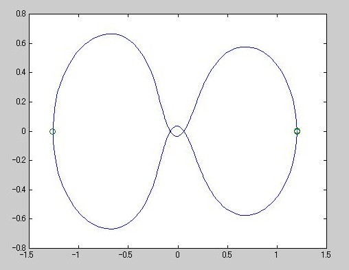
 》 type orbitode
function varargout = orbitode(t,y,flag)
%ORBITODE Restricted 3 body problem.
% This is a standard test problem for non-stiff solvers stated in Shampine
% and Gordon, p. 246 ff. The first two solution components are
% coordinates of the body of infinitesimal mass, so plotting one against
% the other gives the orbit of the body around the other two bodies. The
% initial conditions have been chosen so as to make the orbit periodic.
% Moderately stringent tolerances are necessary to reproduce the
% qualitative behavior of the orbit. Suitable values are 1e-5 for RelTol
% and and 1e-4 for AbsTol.
%
% ORBITDEM with no input arguments runs a demo of event location where the
% ability to specify the direction of the zero crossing is critical. Both
% the point of return to the initial point and the point of maximum
% distance have the same event function value, and the direction of the
% crossing is used to distinguish them.
%
% L. F. Shampine and M. K. Gordon, Computer Solution of Ordinary
% Differential Equations, W.H. Freeman & Co., 1975.
%
% See also ODE45, ODE23, ODE113, ODESET, ODEFILE.
% Mark W. Reichelt and Lawrence F. Shampine, 3-23-94, 4-19-94
% Copyright (c) 1984-98 by The MathWorks, Inc.
% $Revision: 1.9 $ $Date: 1997/11/21 23:26:42 $
y0 = [1.2; 0; 0; -1.04935750983031990726];
if nargin == 0
flag = 'demo';
end
switch flag
case '' % Return dy/dt = f(t,y).
varargout{1} = f(t,y);
case 'init' % Return default [tspan,y0,options].
[varargout{1:3}] = init(y0);
case 'events' % Return [value,isterminal,direction].
[varargout{1:3}] = events(t,y,y0);
case 'demo' % Run a demo.
demo;
otherwise
error(['Unknown flag ''' flag '''.']);
end
% --------------------------------------------------------------------------
function dydt = f(t,y)
mu = 1 / 82.45;
mustar = 1 - mu;
r13 = ((y(1) + mu)^2 + y(2)^2) ^ 1.5;
r23 = ((y(1) - mustar)^2 + y(2)^2) ^ 1.5;
dydt = [ y(3)
y(4)
(2*y(4) + y(1) - mustar*((y(1)+mu)/r13) - mu*((y(1)-mustar)/r23))
(-2*y(3) + y(2) - mustar*(y(2)/r13) - mu*(y(2)/r23)) ];
% --------------------------------------------------------------------------
function [tspan,y0,options] = init(y)
tspan = [0; 6.19216933131963970674];
y0 = y;
options = odeset('RelTol',1e-5,'AbsTol',1e-4);
% --------------------------------------------------------------------------
function [value,isterminal,direction] = events(t,y,y0)
% Locate the time when the object returns closest to the initial point y0
% and starts to move away, and stop integration. Also locate the time when
% the object is farthest from the initial point y0 and starts to move closer.
%
% The current distance of the body is
%
% DSQ = (y(1)-y0(1))^2 + (y(2)-y0(2))^2 = <y(1:2)-y0,y(1:2)-y0>
%
% A local minimum of DSQ occurs when d/dt DSQ crosses zero heading in
% the positive direction. We can compute d/dt DSQ as
%
% d/dt DSQ = 2*(y(1:2)-y0)'*dy(1:2)/dt = 2*(y(1:2)-y0)'*y(3:4)
%
dDSQdt = 2 * ((y(1:2)-y0(1:2))' * y(3:4));
value = [dDSQdt; dDSQdt];
isterminal = [1; 0]; % stop at local minimum
direction = [1; -1]; % [local minimum, local maximum]
% --------------------------------------------------------------------------
function demo
fprintf('\nThis is an example of event location where the ability to\n');
fprintf('specify the direction of the zero crossing is critical. Both\n');
fprintf('the point of return to the initial point and the point of\n');
fprintf('maximum distance have the same event function value, and the\n');
fprintf('direction of the crossing is used to distinguish them.\n\n');
fprintf('Calling ODE45 on ORBITODE with event functions active...\n\n');
fprintf('Note that the step sizes used by the integrator are NOT\n');
fprintf('determined by the location of the events, and the events are\n');
fprintf('still located accurately.\n\n');
options = odeset('Events','on','OutputFcn','odephas2');
[t,y,te,ye,ie] = ode45('orbitode',[0;10],[],options);
plot(y(:,1),y(:,2),ye(:,1),ye(:,2),'o');
》 orbitode
This is an example of event location where the ability to
specify the direction of the zero crossing is critical. Both
the point of return to the initial point and the point of
maximum distance have the same event function value, and the
direction of the crossing is used to distinguish them.
Calling ODE45 on ORBITODE with event functions active...
Note that the step sizes used by the integrator are NOT
determined by the location of the events, and the events are
still located accurately.
》 type orbitode
function varargout = orbitode(t,y,flag)
%ORBITODE Restricted 3 body problem.
% This is a standard test problem for non-stiff solvers stated in Shampine
% and Gordon, p. 246 ff. The first two solution components are
% coordinates of the body of infinitesimal mass, so plotting one against
% the other gives the orbit of the body around the other two bodies. The
% initial conditions have been chosen so as to make the orbit periodic.
% Moderately stringent tolerances are necessary to reproduce the
% qualitative behavior of the orbit. Suitable values are 1e-5 for RelTol
% and and 1e-4 for AbsTol.
%
% ORBITDEM with no input arguments runs a demo of event location where the
% ability to specify the direction of the zero crossing is critical. Both
% the point of return to the initial point and the point of maximum
% distance have the same event function value, and the direction of the
% crossing is used to distinguish them.
%
% L. F. Shampine and M. K. Gordon, Computer Solution of Ordinary
% Differential Equations, W.H. Freeman & Co., 1975.
%
% See also ODE45, ODE23, ODE113, ODESET, ODEFILE.
% Mark W. Reichelt and Lawrence F. Shampine, 3-23-94, 4-19-94
% Copyright (c) 1984-98 by The MathWorks, Inc.
% $Revision: 1.9 $ $Date: 1997/11/21 23:26:42 $
y0 = [1.2; 0; 0; -1.04935750983031990726];
if nargin == 0
flag = 'demo';
end
switch flag
case '' % Return dy/dt = f(t,y).
varargout{1} = f(t,y);
case 'init' % Return default [tspan,y0,options].
[varargout{1:3}] = init(y0);
case 'events' % Return [value,isterminal,direction].
[varargout{1:3}] = events(t,y,y0);
case 'demo' % Run a demo.
demo;
otherwise
error(['Unknown flag ''' flag '''.']);
end
% --------------------------------------------------------------------------
function dydt = f(t,y)
mu = 1 / 82.45;
mustar = 1 - mu;
r13 = ((y(1) + mu)^2 + y(2)^2) ^ 1.5;
r23 = ((y(1) - mustar)^2 + y(2)^2) ^ 1.5;
dydt = [ y(3)
y(4)
(2*y(4) + y(1) - mustar*((y(1)+mu)/r13) - mu*((y(1)-mustar)/r23))
(-2*y(3) + y(2) - mustar*(y(2)/r13) - mu*(y(2)/r23)) ];
% --------------------------------------------------------------------------
function [tspan,y0,options] = init(y)
tspan = [0; 6.19216933131963970674];
y0 = y;
options = odeset('RelTol',1e-5,'AbsTol',1e-4);
% --------------------------------------------------------------------------
function [value,isterminal,direction] = events(t,y,y0)
% Locate the time when the object returns closest to the initial point y0
% and starts to move away, and stop integration. Also locate the time when
% the object is farthest from the initial point y0 and starts to move closer.
%
% The current distance of the body is
%
% DSQ = (y(1)-y0(1))^2 + (y(2)-y0(2))^2 = <y(1:2)-y0,y(1:2)-y0>
%
% A local minimum of DSQ occurs when d/dt DSQ crosses zero heading in
% the positive direction. We can compute d/dt DSQ as
%
% d/dt DSQ = 2*(y(1:2)-y0)'*dy(1:2)/dt = 2*(y(1:2)-y0)'*y(3:4)
%
dDSQdt = 2 * ((y(1:2)-y0(1:2))' * y(3:4));
value = [dDSQdt; dDSQdt];
isterminal = [1; 0]; % stop at local minimum
direction = [1; -1]; % [local minimum, local maximum]
% --------------------------------------------------------------------------
function demo
fprintf('\nThis is an example of event location where the ability to\n');
fprintf('specify the direction of the zero crossing is critical. Both\n');
fprintf('the point of return to the initial point and the point of\n');
fprintf('maximum distance have the same event function value, and the\n');
fprintf('direction of the crossing is used to distinguish them.\n\n');
fprintf('Calling ODE45 on ORBITODE with event functions active...\n\n');
fprintf('Note that the step sizes used by the integrator are NOT\n');
fprintf('determined by the location of the events, and the events are\n');
fprintf('still located accurately.\n\n');
options = odeset('Events','on','OutputFcn','odephas2');
[t,y,te,ye,ie] = ode45('orbitode',[0;10],[],options);
plot(y(:,1),y(:,2),ye(:,1),ye(:,2),'o');
》 orbitode
This is an example of event location where the ability to
specify the direction of the zero crossing is critical. Both
the point of return to the initial point and the point of
maximum distance have the same event function value, and the
direction of the crossing is used to distinguish them.
Calling ODE45 on ORBITODE with event functions active...
Note that the step sizes used by the integrator are NOT
determined by the location of the events, and the events are
still located accurately.
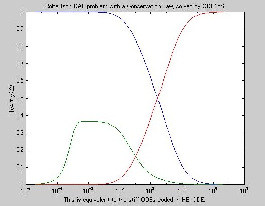
function varargout = hb1dae(t,y,flag)
%HB1DAE Stiff differential-algebraic equation (DAE) from a conservation law.
% HB1DAE with no input arguments runs a demo of the solution of a stiff
% differential-algebraic equation (DAE) system expressed as a problem with
% a singular mass matrix, M*y' = f(t,y).
%
% The Robertson problem coded in HB1ODE is a classic test problem for
% codes that solve stiff ODEs. The problem is
%
% y(1)' = -0.04*y(1) + 1e4*y(2)*y(3)
% y(2)' = 0.04*y(1) - 1e4*y(2)*y(3) - 3e7*y(2)^2
% y(3)' = 3e7*y(2)^2
%
% It is to be solved with initial conditions y(1) = 1, y(2) = 0, y(3) = 0
% to steady state.
%
% These differential equations satisfy a linear conservation law that can
% be used to reformulate the problem as the DAE
%
% y(1)' = -0.04*y(1) + 1e4*y(2)*y(3)
% y(2)' = 0.04*y(1) - 1e4*y(2)*y(3) - 3e7*y(2)^2
% 0 = y(1) + y(2) + y(3) - 1
%
% This problem is used as an example in the prolog to LSODI [1]. Though
% consistent initial conditions are obvious, the guess y(3) = 1e-3 is used
% to test initialization. A logarithmic scale is appropriate for plotting
% the solution on the long time interval. y(2) is small and its major
% change takes place in a relatively short time. Accordingly, the prolog
% to LSODI specifies a much smaller absolute error tolerance on this
% component. Also, when plotting it with the other components, it is
% multiplied by 1e4. The natural output of the code does not show clearly
% the behavior of this component, so additional output is specified for
% this purpose.
%
% [1] A.C. Hindmarsh, LSODE and LSODI, two new initial value ordinary
% differential equation solvers, SIGNUM Newsletter, 15 (1980),
% pp. 10-11.
%
% See also ODE15S, ODE23T, ODESET, ODEFILE, HB1ODE, AMP1DAE.
% Mark W. Reichelt and Lawrence F. Shampine, 3-6-98
% Copyright (c) 1984-98 by The MathWorks, Inc.
% $Revision: 1.3 $
if nargin == 0
flag = 'demo';
end
switch flag
case '' % Return dy/dt = f(t,y).
varargout{1} = f(t,y);
case 'init' % Return default [tspan,y0,options].
[varargout{1:3}] = init;
case 'mass' % Return mass matrix M.
varargout{1} = mass;
case 'demo' % Run a demo.
demo;
otherwise
error(['Unknown flag ''' flag '''.']);
end
% --------------------------------------------------------------------------
function dydt = f(t,y)
dydt = [ (-0.04*y(1,:) + 1e4*y(2,:).*y(3,:))
(0.04*y(1,:) - 1e4*y(2,:).*y(3,:) - 3e7*y(2,:).^2)
(y(1,:) + y(2,:) + y(3,:) - 1) ];
% --------------------------------------------------------------------------
function [tspan,y0,options] = init
tspan = [0 4*logspace(-6,6)];
% Note that this is an inconsistent initial condition.
y0 = [1; 0; 1e-3];
% The tolerances are those of the LSODI example.
options = odeset('Mass','M','MassSingular','yes','RelTol',1e-4, ...
'AbsTol',[1e-6 1e-10 1e-6],'Vectorized','on');
% --------------------------------------------------------------------------
function M = mass(t,y)
M = [1 0 0; 0 1 0; 0 0 0];
% --------------------------------------------------------------------------
function demo
% Use an inconsistent initial condition to test initialization.
y0 = [1; 0; 1e-3];
% Use the LSODI example tolerances. The 'MassSingular' property is
% left at its default 'maybe' to test the automatic detection of a DAE.
options = odeset('Mass','M','RelTol',1e-4,'AbsTol',[1e-6 1e-10 1e-6], ...
'Vectorized','on');
[t,y] = ode15s('hb1dae',[0 4*logspace(-6,6)],y0,options);
y(:,2) = 1e4*y(:,2);
semilogx(t,y)
ylabel('1e4 * y(:,2)')
title('Robertson DAE problem with a Conservation Law, solved by ODE15S')
xlabel('This is equivalent to the stiff ODEs coded in HB1ODE.')
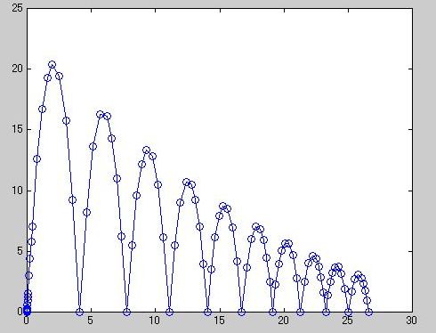
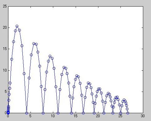
》 type ballode.m
function varargout = ballode(t,y,flag)
%BALLODE Equations of motion for a bouncing ball.
% BALLODE(T,Y) returns the derivatives vector for the equations of motion
% for a bouncing ball. This ODE file can be used to test the
% zero-crossing location capabilities of the ODE Suite solvers.
%
% BALLODE(T,Y,'events') returns a zero-crossing vector VALUE evaluated at
% (T,Y) and two constant vectors ISTERMINAL and DIRECTION. By default,
% the solvers of the ODE Suite do not locate zero-crossings. However, if
% the ODE solver property Events is set to 'on' with ODESET, the solver
% calls the ODE file with the flag 'events'. The ODE file returns the
% information that the solver uses to locate zero-crossings of the
% elements in the VALUE vector. The VALUE vector may be of any length.
% It is evaluated at the beginning and end of a step, and if any elements
% make transitions to, from, or through zero (with the directionality
% specified in DIRECTION), then the zero-crossing point is located. The
% ISTERMINAL vector consists of logical 1's and 0's, enabling you to
% specify whether or not a zero-crossing of the corresponding VALUE
% element halts the integration. The DIRECTION vector enables you to
% specify a desired directionality, positive (1), negative (-1), and don't
% care (0) for each VALUE element.
%
% BALLODE(T,Y,'init') returns initial conditions (see RIGIDODE).
%
% BALLODE with no input arguments runs a demo of a bouncing ball. It is
% an example of repeated event location, where the initial conditions are
% changed after each terminal event. This demo computes ten bounces with
% calls to ODE45. The speed of the ball is attenuated by 0.9 after each
% bounce, and the simulation is stopped when the time for a bounce has
% decreased to a minimum length. Note that the event function also
% locates the peak of each bounce.
%
% See also ODE45, ODESET, ODEFILE.
% Mark W. Reichelt and Lawrence F. Shampine, 1/3/95
% Copyright (c) 1984-98 by The MathWorks, Inc.
% $Revision: 1.10 $ $Date: 1997/11/21 23:25:02 $
if nargin == 0
flag = 'demo';
end
switch flag
case '' % Return dy/dt = f(t,y).
varargout{1} = f(t,y);
case 'init' % Return default [tspan,y0,options].
[varargout{1:3}] = init;
case 'events' % Return [value,isterminal,direction].
[varargout{1:3}] = events(t,y);
case 'demo' % Run a demo.
demo;
otherwise
error(['Unknown flag ''' flag '''.']);
end
% --------------------------------------------------------------------------
function dydt = f(t,y)
dydt = [y(2); -9.8];
% --------------------------------------------------------------------------
function [tspan,y0,options] = init
tspan = [0; 10];
y0 = [0; 20];
options = odeset('Events','on');
% --------------------------------------------------------------------------
function [value,isterminal,direction] = events(t,y)
% Locate the time when height passes through zero in a decreasing direction
% and stop integration. Also locate both decreasing and increasing
% zero-crossings of velocity, and don't stop integration.
value = y; % [height; velocity]
isterminal = [1; 0];
direction = [-1; 0];
% --------------------------------------------------------------------------
function demo
tstart = 0;
tfinal = 30;
y0 = [0; 20];
refine = 4;
options = odeset('Events','on','OutputFcn','odeplot','OutputSel',1,...
'Refine',refine);
clf reset % deletes any stop button
set(gca,'xlim',[0 30],'ylim',[0 25]);
box on
hold on;
tout = tstart;
yout = y0.';
teout = [];
yeout = [];
ieout = [];
for i = 1:10
% Solve until the first terminal event.
[t,y,te,ye,ie] = ode23('ballode',[tstart tfinal],y0,options);
if ~ishold
hold on
end
% Accumulate output. This could be passed out as output arguments.
nt = length(t);
tout = [tout; t(2:nt)];
yout = [yout; y(2:nt,:)];
teout = [teout; te]; % Events at tstart are never reported.
yeout = [yeout; ye];
ieout = [ieout; ie];
ud = get(gcf,'UserData');
if ud.stop
break;
end
% Set the new initial conditions, with .9 attenuation.
y0(1) = 0;
y0(2) = -.9*y(nt,2);
% A good guess of a valid first timestep is the length of the last valid
% timestep, so use it for faster computation. 'refine' is 4 by default.
options = odeset(options,'InitialStep',t(nt)-t(nt-refine),...
'MaxStep',t(nt)-t(1));
tstart = t(nt);
end
hold off
odeplot([],[],'done');
》 ballode
》
返回